Estimating Policy Barriers to Trade
22 November 2019
Brendan Cooley
Ph.D. Candidate
Princeton University
bcooley (at) princeton.edu
The Tariff System (GATT/WTO)
- Free? Applied tariff rates are low, ~5% on average (Baldwin 2016)
- Fair? WTO members (vast majority of world economy) commit to principle of non-discrimination (Most Favored Nation)
The Tariff System (GATT/WTO)
- Free? Applied tariff rates are low, ~5% on average (Baldwin 2016)
- Fair? WTO members (vast majority of world economy) commit to principle of non-discrimination (Most Favored Nation)
Measurement Matters
Measurement Matters
Prices and Trade Costs
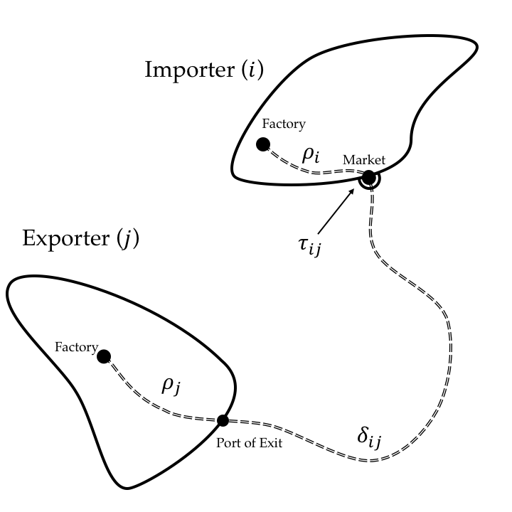
\[ p_{ji}(\omega) = d_{ji} p_{ii}(\omega) \]
\[ d_{ij} = \rho_j \delta_{ij} \tau_{ij} \]
- \(\tau_{ij} = 1 \implies\) no policy distortion
- \(\tau_{jj} = \delta_{jj} = 1\)
\[ p_i^\star(\omega) = \min_{j \in \left\{ 1,...,N \right\}} \left\{ p_{ij} \right\} \]
\[ \Omega_{ij}^\star = \left\{ \omega \in [0,1] \text{ } \bigg| \text{ } p_{ij}(\omega) \leq \min_{k \neq j} \left\{ p_{ik} \right\} \right\} \]
Preliminary Evidence of Significant Barriers
Preliminary Evidence of Significant Barriers
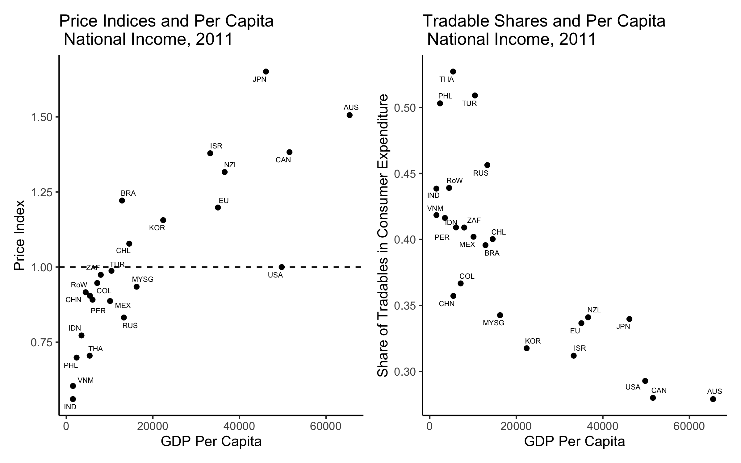
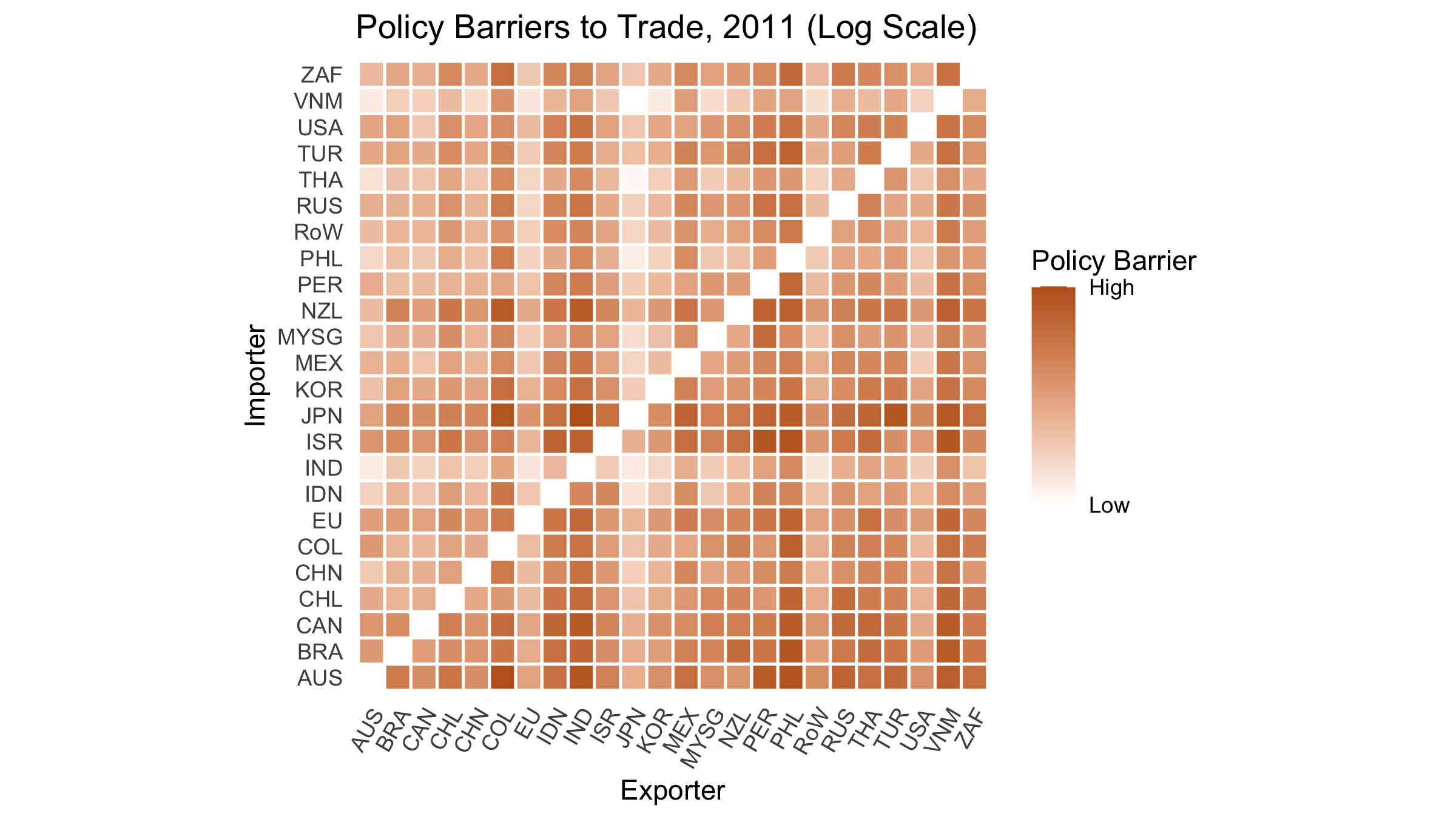
Price Levels (Estimates)
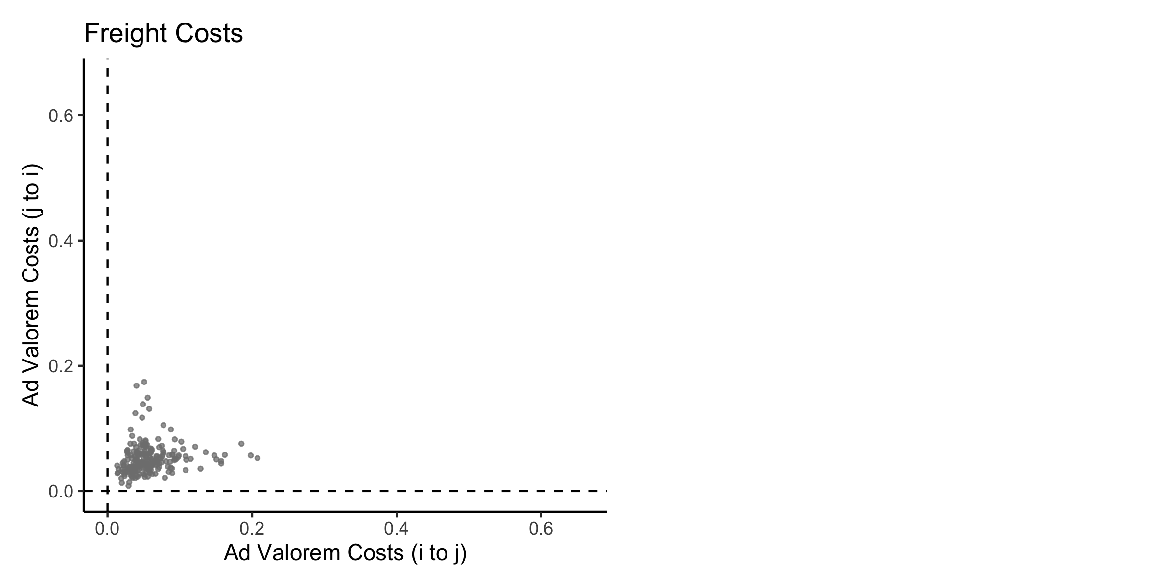
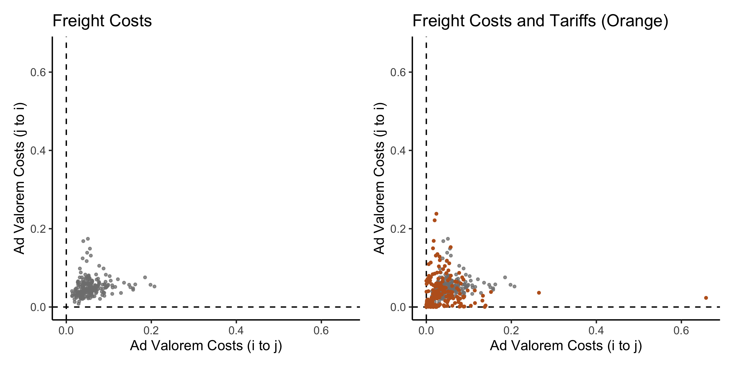
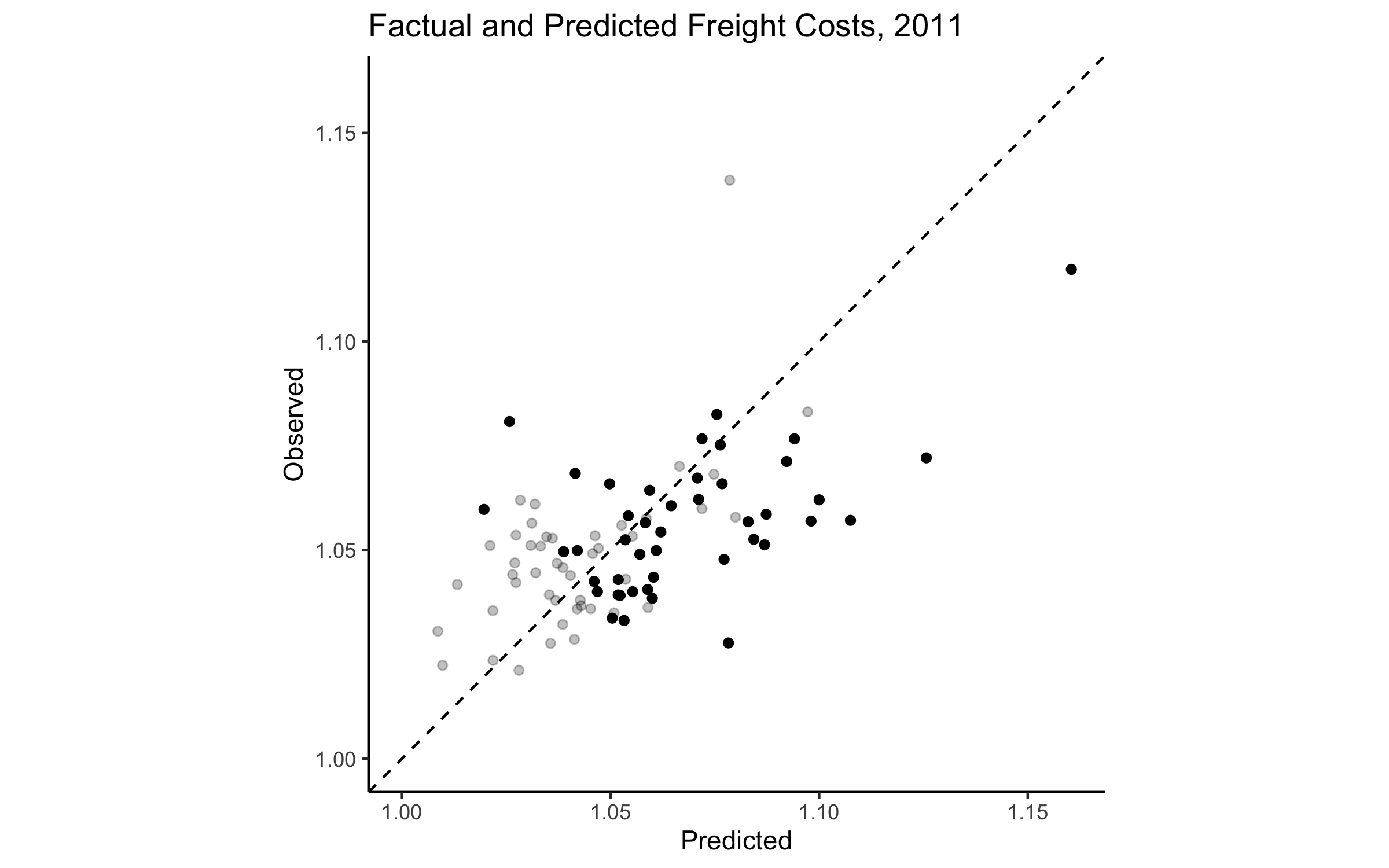
Freight Costs (Cross Validation)
Results
Results
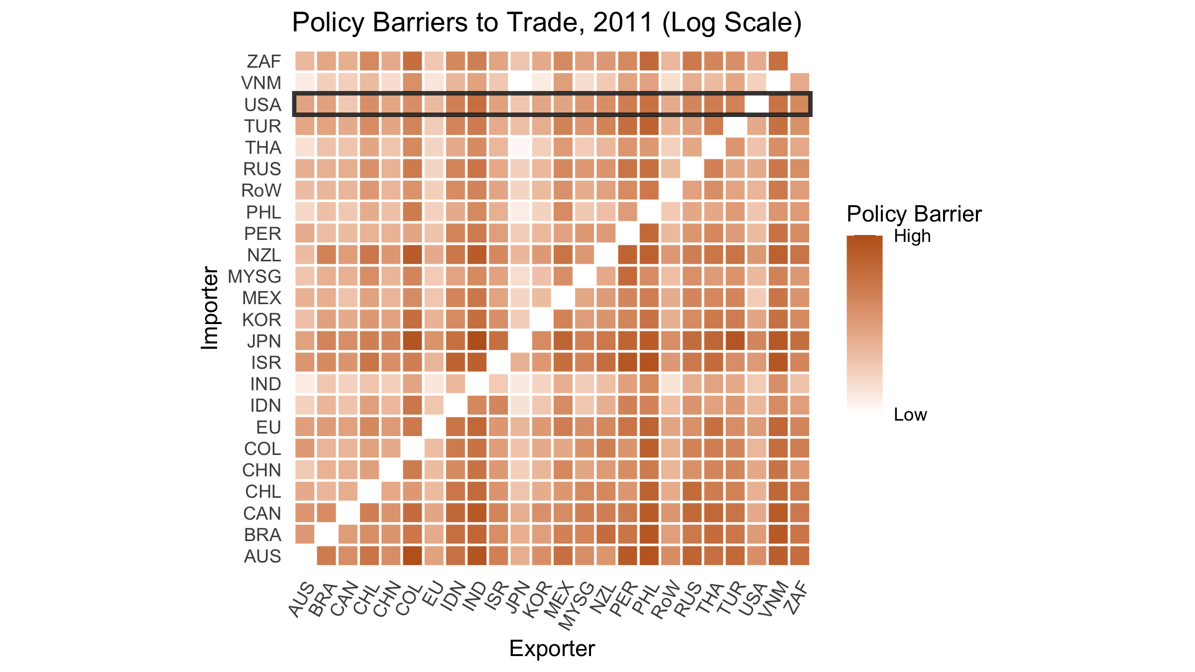
- U.S. favored partners: Canada (19% ad valorem), Japan (21%), EU (40%)
- U.S. disfavored partners: Peru (211%) and Vietnam (260%)
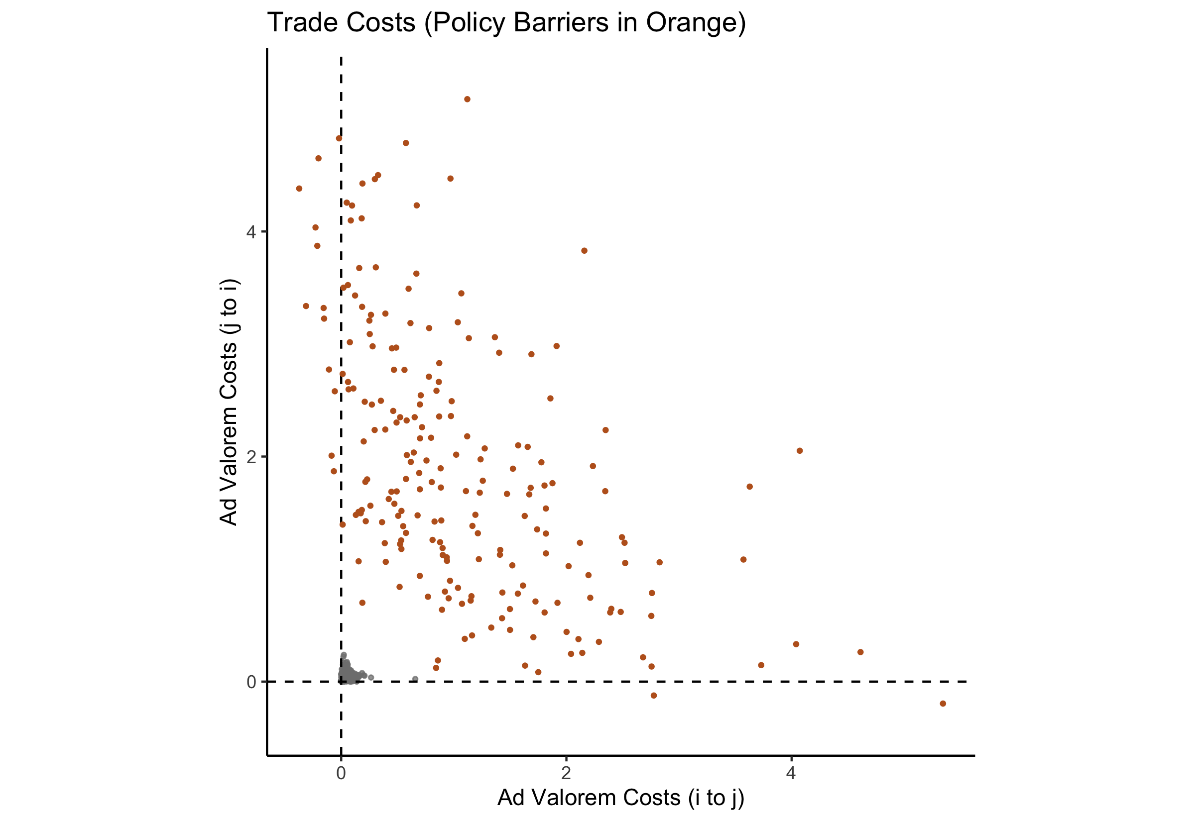
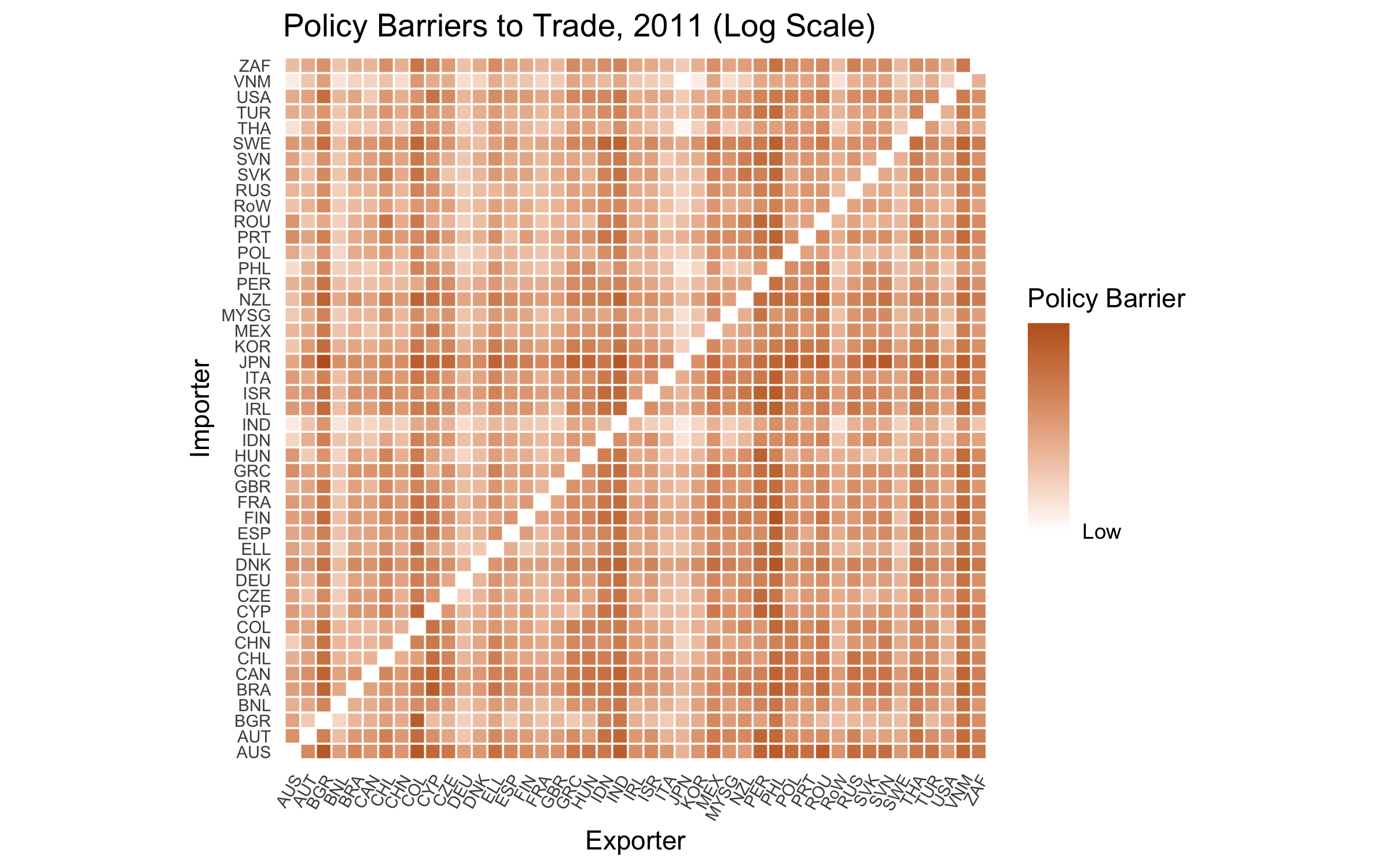
Results (Free?)
Results (Free?)
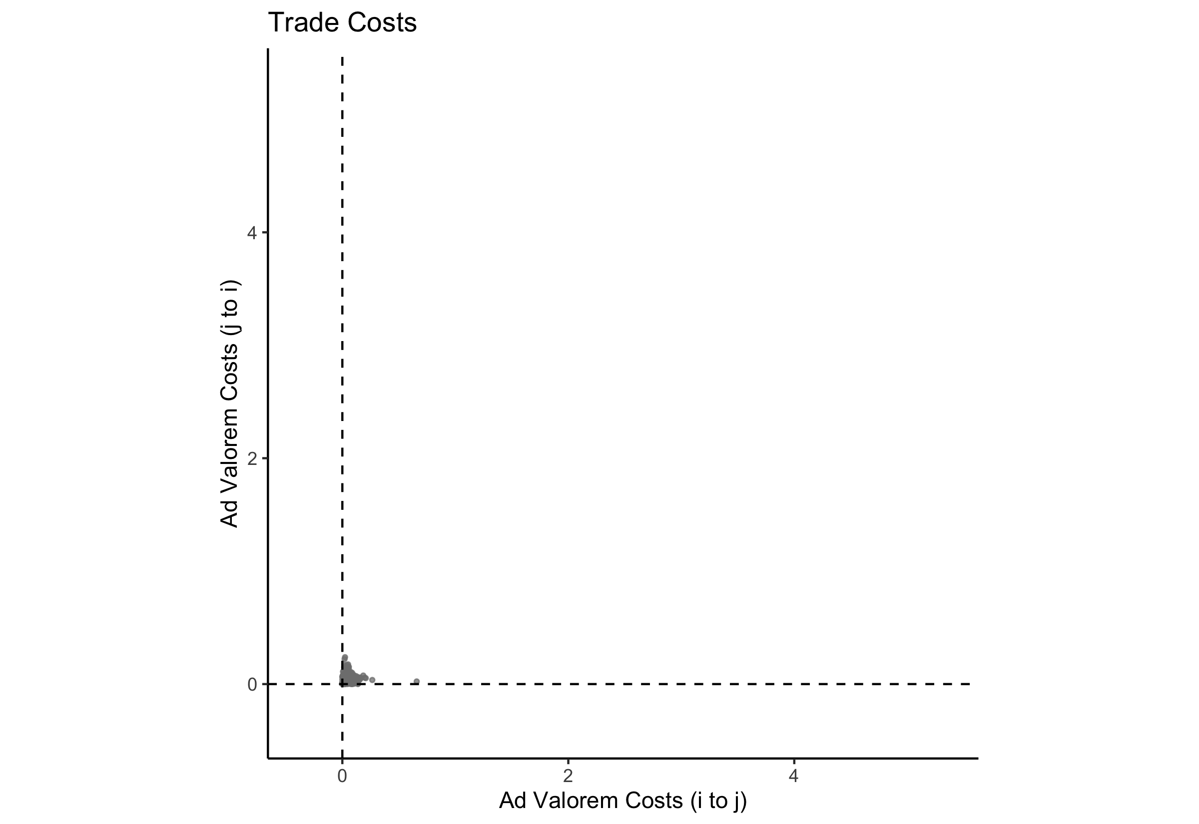
Results (Free?)
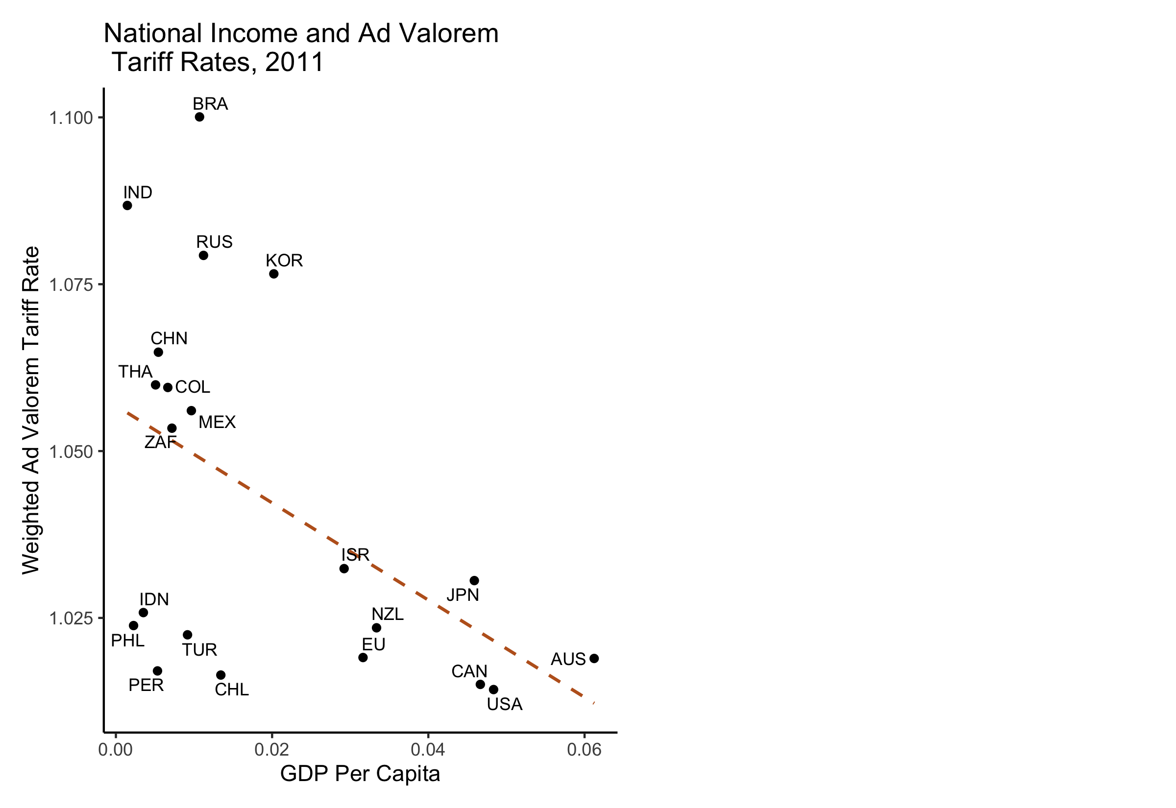
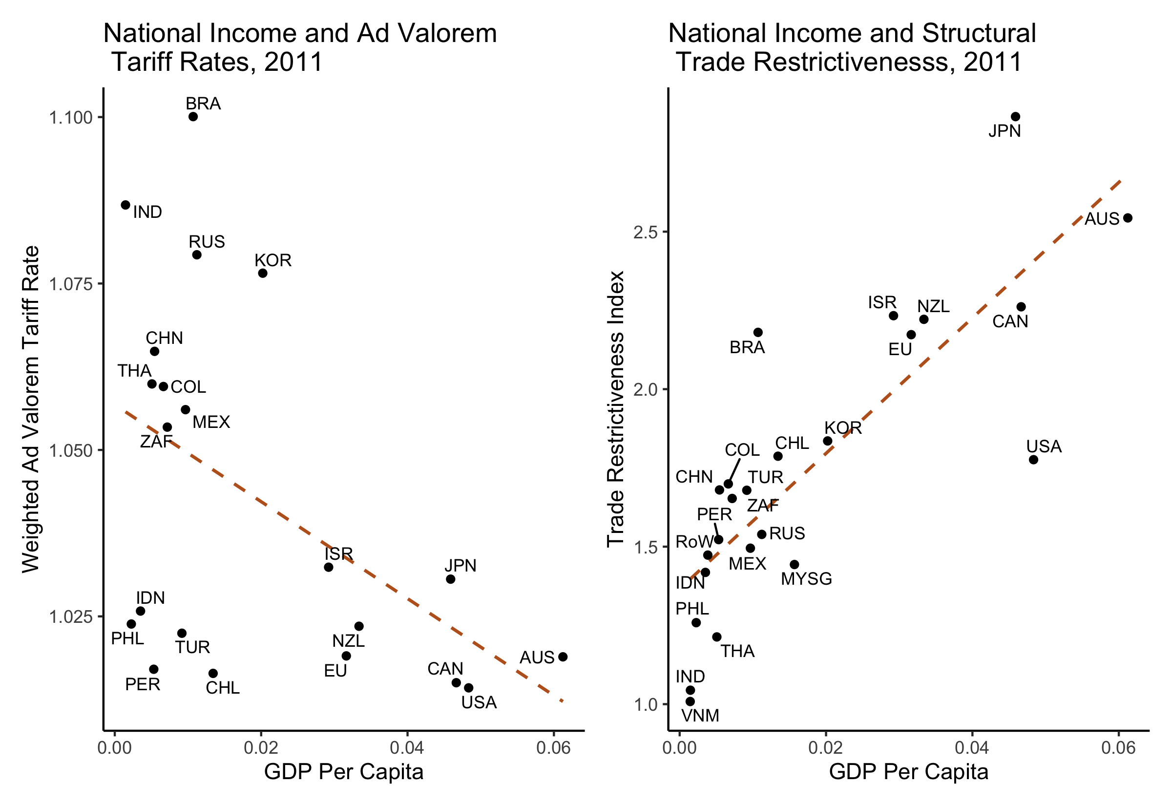
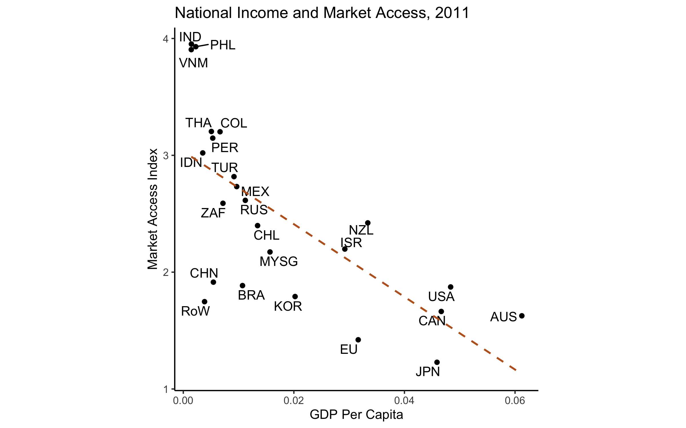
Results (Fair?)
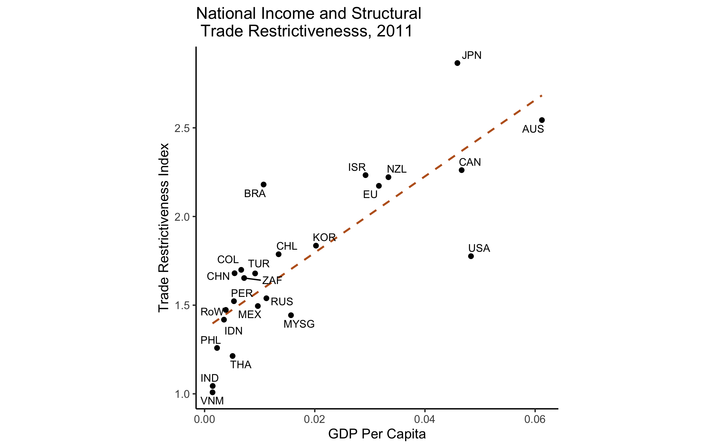
Results (Fair?)
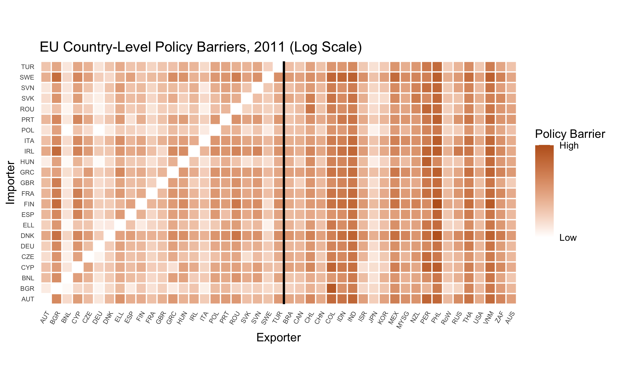
Robustness (Intra-European Barriers)
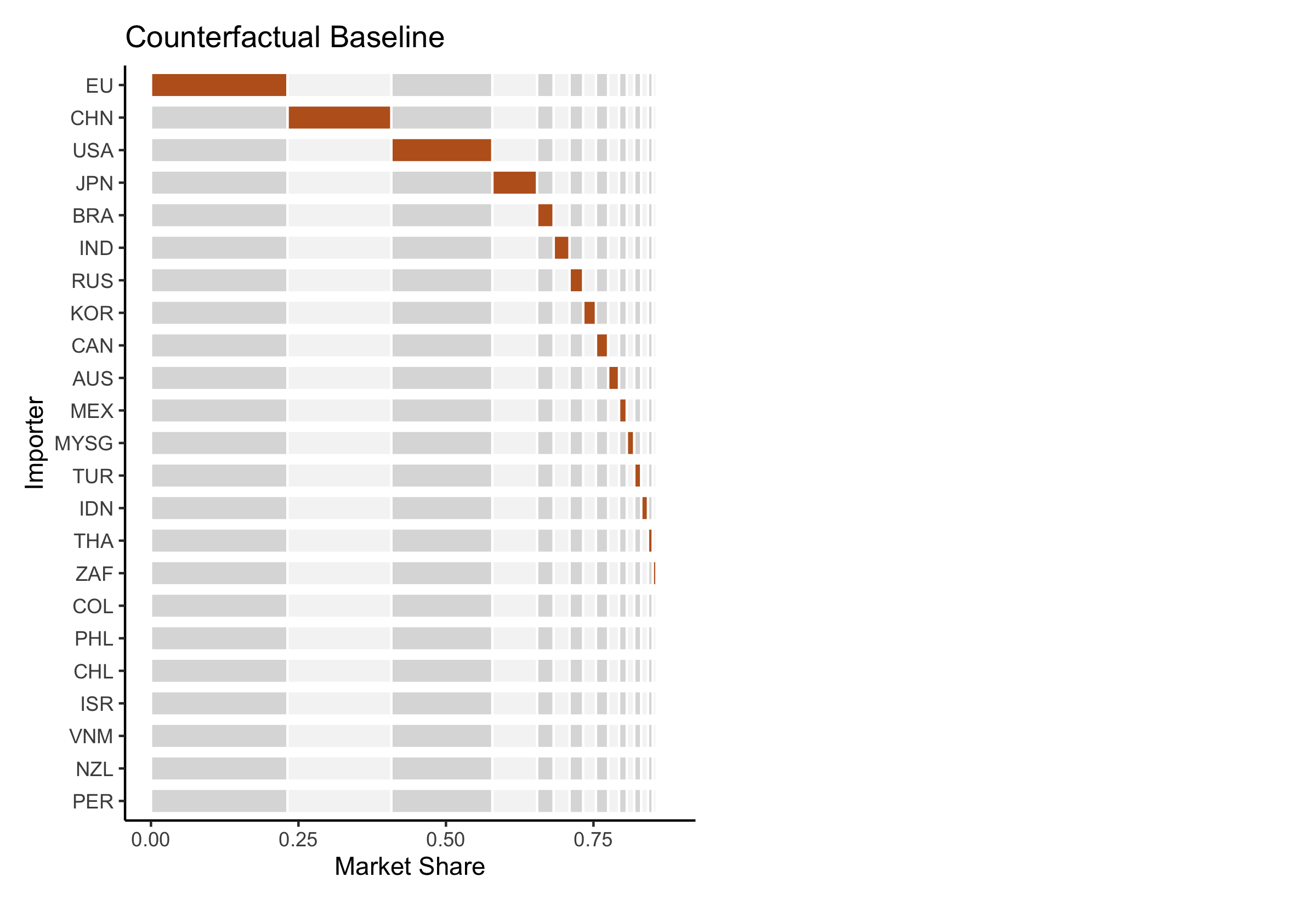
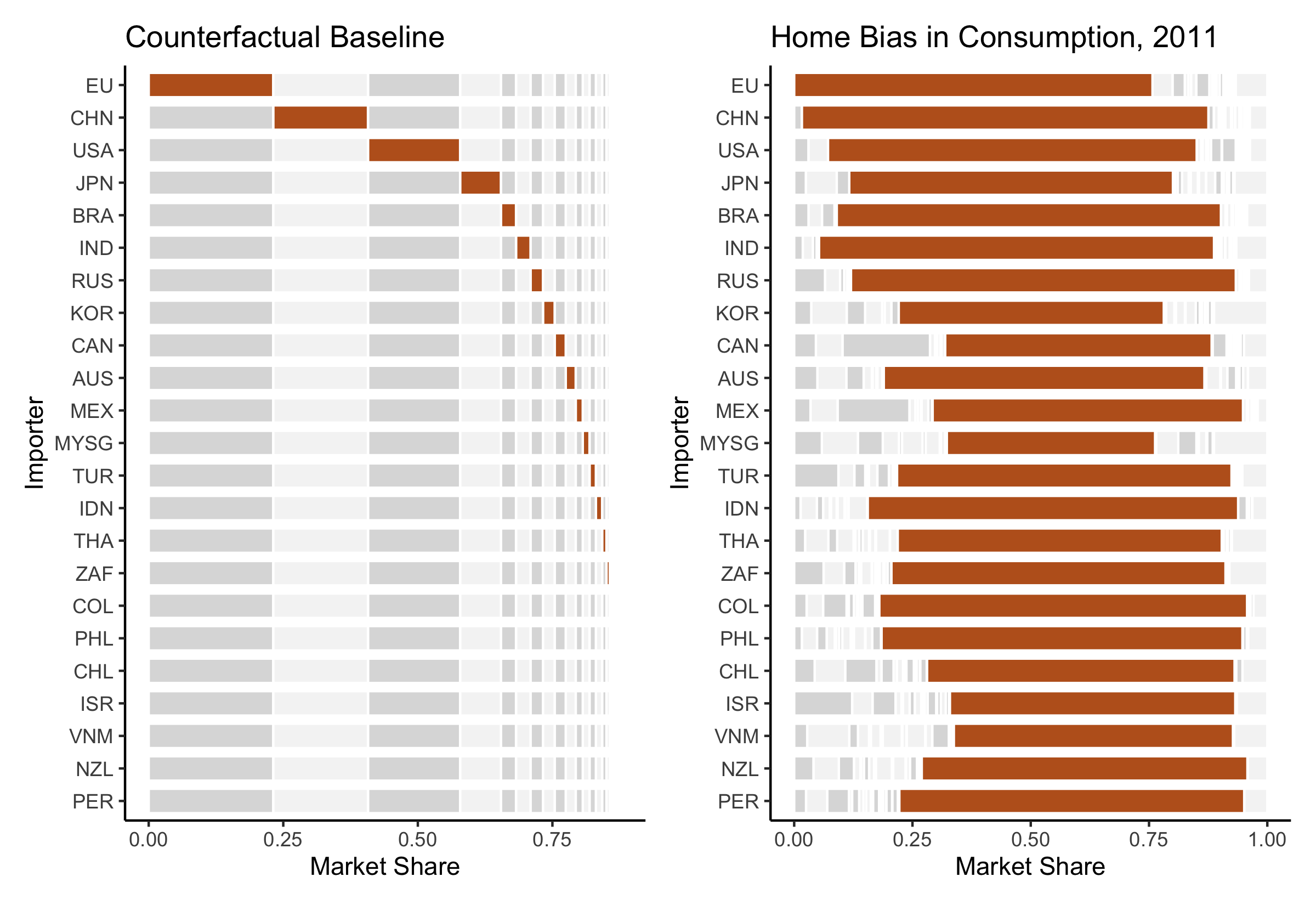
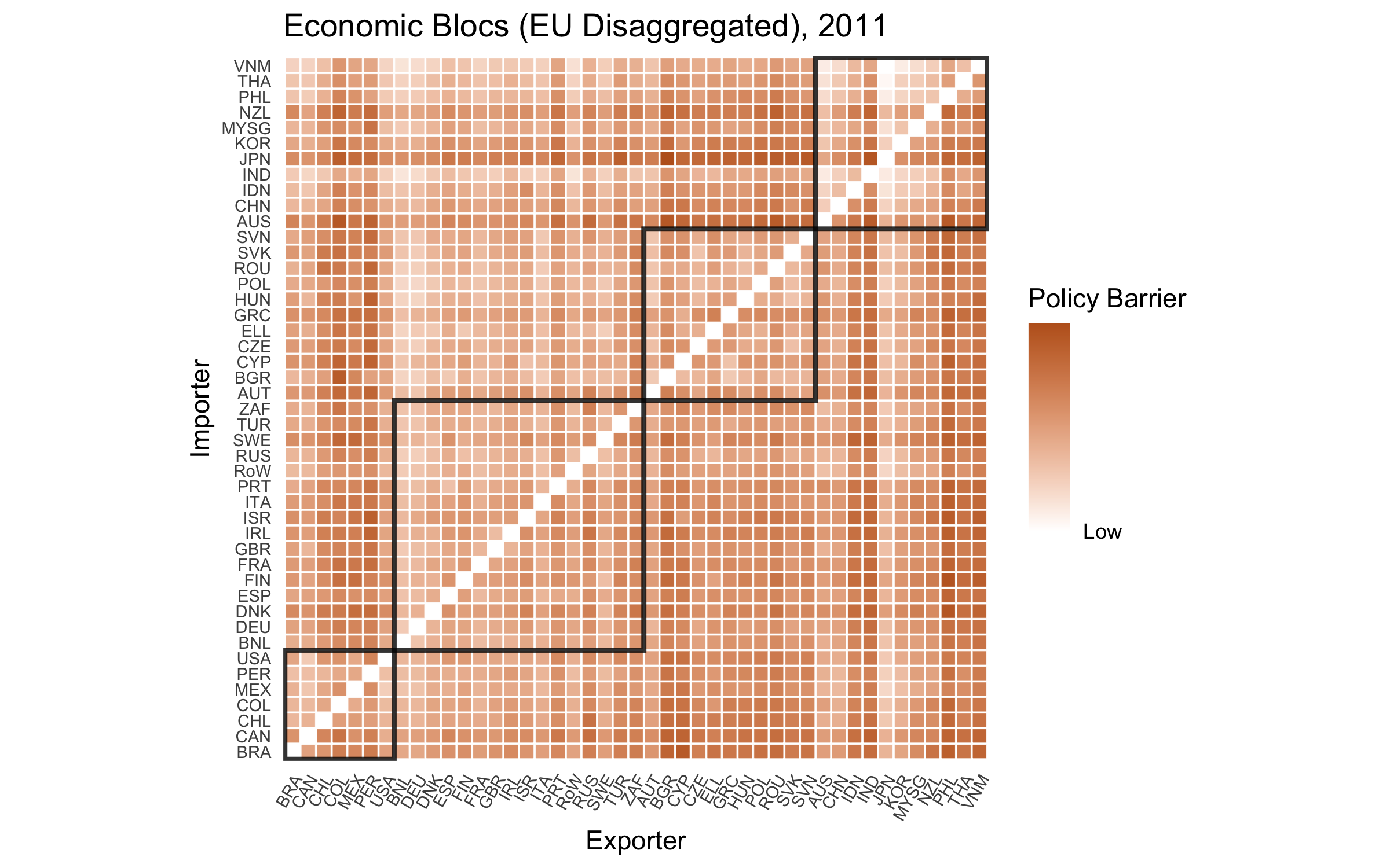
Implications (Economic Blocs)
Implications (Economic Blocs)
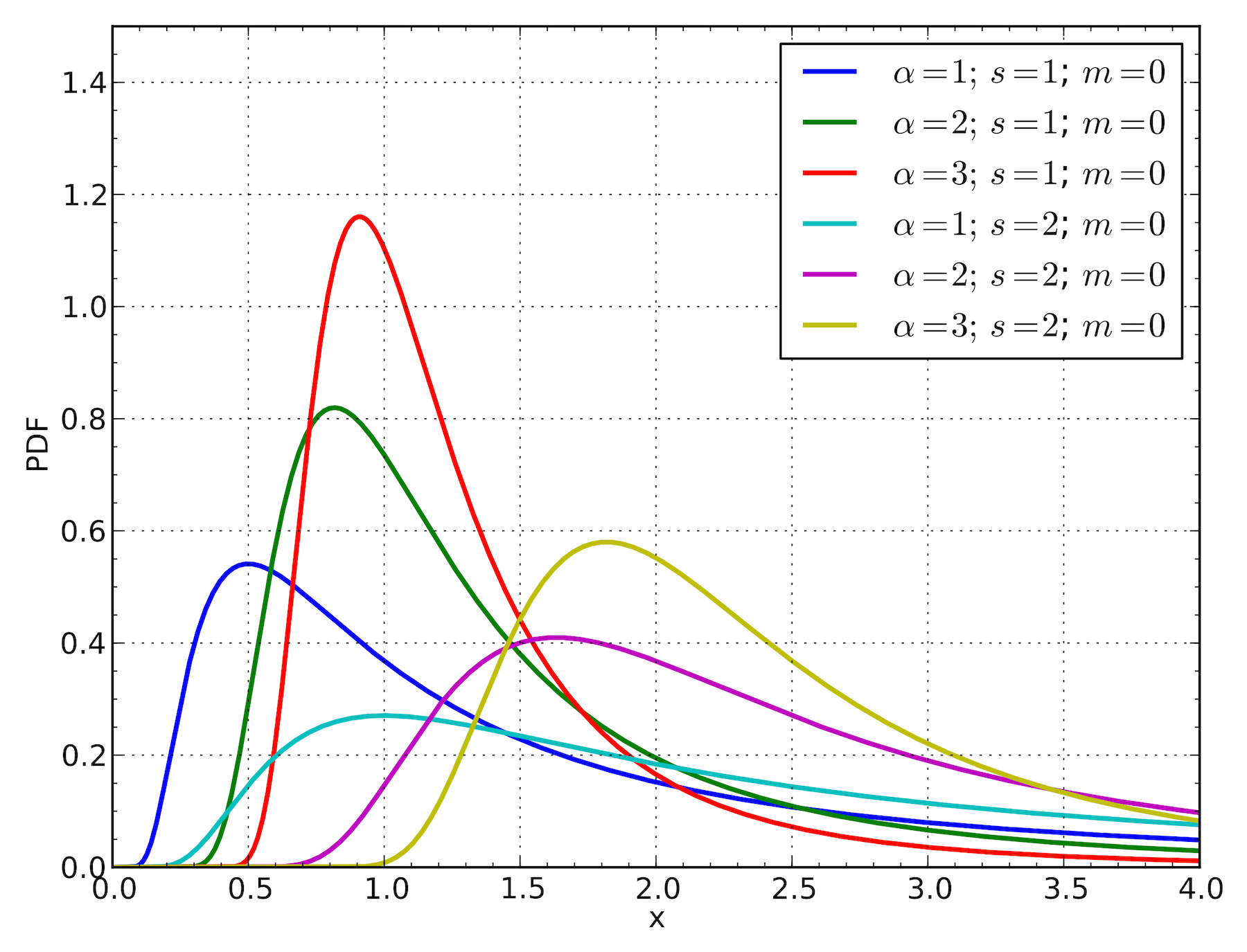
Fréchet Distribution
Acemoglu, Daron. 2005. “Politics and economics in weak and strong states.” Journal of Monetary Economics 52 (7): 1199–1226.
Alvarez, Fernando, and Robert E Lucas. 2007. “General equilibrium analysis of the Eaton–Kortum model of international trade.” Journal of Monetary Economics 54: 1726–68.
Anderson, James E, and Eric Van Wincoop. 2003. “Gravity with Gravitas: A Solution to the Border Puzzle.” The American Economic Review 93 (1): 170–92.
Baccini, Leonardo. 2019. “The Economics and Politics of Preferential Trade Agreements.” Annual Review of Political Science 22.
Bagwell, Kyle, and Robert W. Staiger. 1999. “An economic theory of GATT.” American Economic Review 89 (1): 215–48.
Baldwin, Richard. 2016. “The World Trade Organization and the Future of Multilateralism.” Journal of Economic Perspectives 30: 95–116.
Barari, Soubhik, In Song Kim, and Weihuang Wong. n.d. “Trade Liberalization and Regime Type: Evidence from a New Tariff-line Dataset.” http://web.mit.edu/insong/www/pdf/poltrade.pdf.
Bown, Chad P. 2004. “Trade policy under the GATT/WTO: empirical evidence of the equal treatment rule.” Canadian Journal of Economics/Revue Canadienne d‘Economique 37 (3): 678–720.
Chaney, Thomas. 2008. “Distorted Gravity: The Intensive and Extensive Margins of International Trade.” American Economic Review 98 (4): 1707–21.
Costinot, Arnaud, and Andrés Rodríguez-Clare. 2015. “Trade Theory with Numbers: Quantifying the Consequences of Globalization.” Handbook of International Economics 4: 197–261.
Eaton, Jonathan, and Samuel Kortum. 2002. “Technology, geography, and trade.” Econometrica 70 (5): 1741–79.
Eichengreen, Barry, and David Leblang. 2008. “Democracy and Globalization.” Economics & Politics 20 (3): 289–334.
Evenett, Simon J., and Bernard Hoekman. 2004. Government Procurement: Market Access, Transparency, and Multilateral Trade Rules. Policy Research Working Papers. The World Bank.
Gawande, Kishore, and Wendy L. Hansen. 1999. “Retaliation, Bargaining, and the Pursuit of "Free and Fair" Trade.” International Organization 53 (1): 117–59.
Gawande, Kishore, Pravin Krishna, and Marcelo Olarreaga. 2009. “What governments maximize and why: the view from trade.” International Organization 63 (03): 491–532.
———. 2015. “A Political-Economic Account of Global Tariffs.” Economics & Politics 27 (2): 204–33.
Head, Keith, and Thierry Mayer. 2014. “Gravity Equations: Workhorse, Toolkit and Cookbook.” In Handbook of International Economics, edited by Elhanan Helpman, G. Gopinath, and K. Rogoff, 4th ed., 131–96.
Kono, Daniel Yuichi. 2006. “Optimal obfuscation: Democracy and trade policy transparency.” American Political Science Review 100 (03): 369–84.
Kono, Daniel Yuichi, and Stephanie J Rickard. 2014. “Buying National: Democracy, Public Procurement, and International Trade.” International Interactions 40 (5): 657–82.
Lee, Jong-Wha, and Phillip Swagel. 1997. “Trade Barriers and Trade Flows Across Countries and Industries.” The Review of Economics and Statistics 79 (3): 372–82.
Maggi, Giovanni. 1999. “The role of multilateral institutions in international trade cooperation.” American Economic Review, 190–214.
Maggi, Giovanni, Monika Mrázová, and J Peter Neary. 2018. “Choked by Red Tape? The Political Economy of Wasteful Trade Barriers.”
Mansfield, Edward D., and Marc L. Busch. 1995. “The Political Economy of Nontariff Barriers: A Cross-National Analysis.” International Organization 49 (4): 723–49.
Melitz, Marc J. 2003. “The impact of trade on intra-industry reallocations and aggregate industry productivity.” Econometrica 71 (6): 1695–1725.
Milner, Helen V, and Keiko Kubota. 2005. “Why the move to free trade? Democracy and trade policy in the developing countries.” International Organization 59 (01): 107–43.
Queralt, Didac. 2015. “From Mercantilism to Free Trade: A History of Fiscal Capacity Building.” Quarterly Journal of Political Science 10: 221–73.
Rickard, Stephanie J. 2012. “A Non-Tariff Protectionist Bias in Majoritarian Politics: Government Subsidies and Electoral Institutions.” International Studies Quarterly 56: 777–85.
Rodrik, Dani. 2008. “Second-Best Institutions.” American Economic Review: Papers & Proceedings 98 (2): 100–104.
Simonovska, Ina, and Michael E Waugh. 2014. “The Elasticity of Trade: Estimates and Evidence.” Journal of International Economics 92 (1): 34–50.
Sposi, Michael. 2015. “Trade barriers and the relative price of tradables.” Journal of International Economics 96 (2): 398–411.
Waugh, Michael E. 2010. “International Trade and Income Differences.” American Economic Review 100: 2093–2124.
Waugh, Michael E, and B Ravikumar. 2016. “Measuring Openness to Trade.” Journal of Economic Dynamics and Control 72: 29–41.